Contents
Abstract
Recent literature questions the transitivity assumption of the Bradley-Terry reward model in RLHF. One approach, called Nash Learning from Human Feedback (NLHF), recasts the alignment problem as a (regularized) two-player zero-sum game. However, algorithms in this line of work are tested on tabular synthetic games generated from uniform random entries without justifying their resemblance to real preference data. Using combinatorial Hodge theory, we quantify the degree of transitivity and cyclicity for both i.i.d. Uniform games and a preference matrix obtained from LMArena, and discover that while the transitive strengths of the games are of the same order, the real game’s cyclic component is 8.6x weaker. We propose a modification to the generator, and find that while the Hodge-matched games accurately track real-game behavior at heavy regularization (\(\beta \ge 0.03\)), they trend in opposite directions as \(\beta\) gets smaller. Finally, we empirically note that the advantage of Extragradient Preference Optimization (EGPO) shows up only when cyclicity is large enough relative to the transitive strength and regularization is weak; at realistic cyclicity, it is not the fastest of the three algorithms we tested.
1. Introduction
RLHF and transitivity. Reinforcement Learning from Human Feedback (RLHF) for Language Model (LM) alignment has emerged as a commercially successful paradigm of reinforcement learning (Szepesvári, 2026). In the original formulation, human preference for LM responses to prompts are assumed to follow the Bradley-Terry (BT) model (Bradley and Terry, 1952), where the odds of one response being preferred over another is exponential in the (linear) difference between the “goodness” of the two responses. BT induces a total order. The validity of the BT model is supported by a long list of applications that long predate RLHF: ELO in Chess, Go, and many competitive video games; Quantal Response Equilibrium (QRE) in economics; and most recently, the empirical success of Proximal Policy Optimization (PPO) (Schulman et al., 2017) and Direct Preference Optimization (DPO) (Rafailov et al., 2023).
However, another list can be compiled of arguments against transitivity in modeling human behavior. Foremost is social choice theory, which contends that human preference can be cyclic due to irrationality or, even when perfect rationality is assumed, simply aggregating population data (May, 1954). Other arguments can be made from the perspectives of law, ecology, and behavioral economics (Klimenko, 2015). More recently, Czarnecki et al. (2020) propose that the geometry of real-world competitive games – rather than being fully transitive or fully cyclic – more so resembles a spinning-top, where the best and worst players follow an essentially transitive ranking, whereas the middling players can form long chains of domination in a cyclic order. This suggests that whether or not real human preference is transitive need not be absolute or clear-cut, and there can be a gradation of cyclicity.
NLHF. Munos et al. (2023) recasts the alignment problem of RLHF into finding the (regularized) Nash equilibrium of a regularized two-player, zero-sum (2p0s) game. More specifically, given two responses (or actions) \(i\) and \(j\), it is postulated that there exists a preference probability \(P(i > j)\) that \(i\) is preferred over \(j\). By tie-breaking arbitrarily we have \(P(i > j) + P(j > i) = 1\). In the simplified, tabular case, we can encode all preference probabilities in a matrix \(P_{ij}\), and the problem of finding the best policy thus amounts to solving a minimax game for the response that performs the best in the worst case against other policies. Regularization comes in the form of a reference policy (which corresponds to the pre-trained policy in PPO). To solve the game, classic online learning algorithms like Online Mirror Descent (OMD) can be used, but a host of other algorithms have also been proposed including NashMD (Munos et al., 2023), Online IPO (Calandriello et al., 2024), and EGPO (Zhou et al., 2025).
The gap. While transitivity can fail in real datasets, it is crucial to understand how badly it fails before deciding which algorithm to choose. Consider the simple example of three responses being preferred over one another: A beats B, B beats C, and C beats A, all by probability \(p\). It is quite plausible for \(p\) to be 55%, which captures a mild preference loop where none of the options is a clear winner. But it is implausible for \(p\) to be 95%. The synthetic games that the tabular experiments in this line of work are tested on are generated with i.i.d. Uniform (or i.i.d. Gaussian), and in either case cycles of the latter type are common. One might surmise that this is an unrealistic assumption that does not translate to real data.
What we did. Using combinatorial Hodge theory introduced by Jiang et al. (2011), we measure the Hodge geometry of a real preference matrix downloaded from LMArena and find it to be far less cyclic than an i.i.d. Uniform preference matrix of the same size. We then build a generator of synthetic games matching the Hodge statistics of the real game and show that it repairs the comparison but only under strong regularization. Moreover, we conclude that among the three algorithms we have tested, OMD is the winner in all cases except in a low-regularization, high-rotation regime which real data doesn’t reach.
2. Framework
Notation. Let \(A\) be the response/action space. In the general case, actions are typically parametrized with a neural network; but in the tabular case, which is more amenable to analysis and simulation, \(A\) is simply a discrete set. Given two actions \(i\) and \(j\), the probability that \(i\) is preferred over \(j\) (with ties broken arbitrarily) is denoted \(P_{ij}\). It is clear that \(P_{ij} + P_{ji} = 1\) and \(P_{ii} = 1/2\).
Let \(\Delta (A) := \{\pi \in \mathbb{R}^{\lvert A\rvert}: 0\le \pi_i\le 1, 1^\top \pi = 1\}\) denote the simplex of policies (distributions) over A. Given two policies \(\pi, \pi' \in \Delta (A)\), the probability that \(\pi\) beats \(\pi'\) is defined as
\[P(\pi > \pi') := E_{i\sim \pi, j\sim \pi'}(P_{ij}) = \sum_{i,j} \pi_i \pi'_j P_{ij} = \pi^\top P \pi'.\]The vanilla preference game is thus defined as
\[\operatorname*{maximize}_\pi \min_{\pi'} \pi^\top P \pi',\]where \(\pi^\top P \pi'\) is the objective for the first player to maximize and the second player to minimize.
Regularized game. In PPO, we base our policy on a pre-trained reference policy \(\pi_{\text{ref}}\) by adding a reverse KL penalty term (Schulman et al., 2017). In NLHF, we base both policies on the same \(\pi_{\text{ref}}\) and penalize them with the same strength \(\beta>0\), leading to the regularized objective (Munos et al., 2023):
\[V(\pi, \pi') := \pi^\top P \pi' - \beta \operatorname{KL}(\pi||\pi_{\text{ref}}) + \beta \operatorname{KL}(\pi'||\pi_{\text{ref}}).\]Note the subtraction for the first player and addition for the second. The regularized game is thus
\[\operatorname*{maximize}_\pi \min_{\pi'} V(\pi, \pi'),\]which has the fixed-point solution (Zhou et al., 2025)
\[\pi^\star \propto \pi_{\text{ref}} \odot \exp(P\pi^\star /\beta).\]which applies to both players since the Nash equilibrium is symmetric (Munos et al., 2023). However, naively iterating on this map is not guaranteed to converge, so we turn to iterative algorithms.
The duality gap is defined as
\[\operatorname{gap}(\pi) = \max_{\pi'} V(\pi',\pi) - \min_{\pi'} V(\pi, \pi').\]Algorithms. We compare three algorithms in NLHF literature. It is convenient to write the tabular policy in softmax form, \(\pi_\theta \propto \exp(\theta)\) with \(\theta \in \mathbb{R}^{\lvert A\rvert}\), and \(\theta_{\text{ref}} := \log \pi_{\text{ref}}\), so that the fixed-point equation reads
\[\theta = \theta_{\text{ref}} + P\pi_\theta/\beta.\]The learning rate is denoted \(\eta\).
Online Mirror Descent (OMD), also, Online IPO. OMD amounts to a damped fixed-point iteration on the equilibrium condition:
\[\theta_{t+1} = \theta_t - \eta\beta\left(\theta_t - \theta_{\text{ref}} - P\pi_t/\beta\right).\]Nash-MD. Due to Munos et al. (2023)
\[\theta_{t+1} = \theta_t - \eta\beta\left(\theta_t - \theta_{\text{ref}} - P\tilde\pi_t/\beta\right).\]EGPO. Zhou et al. (2025) consider the extragradient: a tentative half-step, then the update repeated from the same base point with the preference re-evaluated at the extrapolated policy.
\[\theta_{t+1/2} = (1-\eta\beta)\theta_t + \eta\beta\left(\theta_{\text{ref}} + P\pi_t/\beta\right),\] \[\theta_{t+1} = (1-\eta\beta)\theta_t + \eta\beta\left(\theta_{\text{ref}} + P\pi_{t+1/2}/\beta\right).\]Note that since each EGPO iteration evaluates \(P\pi\) twice (or, in the neural network case, requires two forward and backward passes) while the other algorithms only need one, it is only fair to charge each EGPO iteration as two steps. Hence in the experiments that follow, EGPO’s steps to convergence is twice its superficial iteration count.
Combinatorial Hodge theory. Combinatorial Hodge theory is a framework developed to extract rankings from graph-based data (Jiang et al., 2011). As it pertains to NLHF, the key insight is that the space of skew-symmetric matrices can be decomposed into the orthogonal sum of the subspace of gradient matrices and the subspace of rotation matrices (Balduzzi et al., 2018), both of which will be defined as follows.
Call an arbitrary vector \(s \in \mathbb{R}^n\) the score vector. Its gradient is defined as
\[\operatorname{grad}(s) := s1^\top - 1s^\top.\]A matrix \(G\) is called a gradient if \(G = \operatorname{grad}(s)\) for some \(s\). Clearly, \(G_{ij} = s_i - s_j\), and \(G\) can thus be interpreted as the flow matrix of a directed graph (that is, \(G_{ij}\) encodes the flow on the edge from node \(i\) to node \(j\)) where the flow is derived from a potential function on the nodes induced by \(s\).
Now let \(Y \in \mathbb{R}^{n \times n}\) be an arbitrary skew-symmetric matrix, and \(W \in \mathbb{R}^{n \times n}\) be a symmetric weight matrix. If \(Y\) is to be construed as an arbitrary flow, then \(W\) should be construed as the weight on each (undirected) edge. We define the score of \(Y\) to be the solution to the following optimization problem:
\[\operatorname*{minimize}_{s\in \mathbb{R}^n} \sum_{i \neq j} w_{ij} (Y_{ij} - (s_i - s_j))^2.\]We define the gradient part of \(Y\) to be the gradient of its score:
\[G := \operatorname{grad}(\operatorname{score}(Y)).\]\(G\) will be, in a sense, the transitive component of \(Y\). We also define the rotational part of \(Y\) to simply be the residual \(R = \operatorname{rot}(Y) := Y - G(Y)\), which will be the cyclic component of \(Y\). The size of \(R\) relative to \(G\) will characterize how “cyclic” a matrix is, in a sense that will be specified below.
We define the weighted inner product between matrices to be \(\langle A,B\rangle_W := \sum W_{ij}A_{ij}B_{ij}\), and the W-norm to be \(\|A\|_W := \langle A, A\rangle_W^{1/2}\).
Theorem (Hodge decomposition, Jiang et al., 2011). \(G \perp R\), in the sense that \(\langle G, R \rangle_W = 0\). Pythagoras also holds, i.e. \(\|G\|_W^2 + \|R\|_W^2 = \|Y\|_W^2\).
The decomposition \(Y = G+R\) is sometimes called the Hodge decomposition and can be computed readily (We give the solution and Python code in Appendix).
Hodge statistics of preference games. Given a preference game \(P \in \mathbb{R}^{n \times n}\), we define its logit-space representation \(Y := \operatorname{logit}(P)\), where \(Y_{ij} := \log (P_{ij}/(1-P_{ij}))\). It is straightforward to verify that \(Y\) is skew-symmetric (use the property \(P_{ij}+P_{ji}=1\)). The reason we choose to work with \(Y\) for defining its cyclicity instead of \(P\) directly is that if the preference probabilities \(P_{ij}\) are generated according to the Bradley-Terry model, that is,
\[P_{ij} = \operatorname{sigmoid}(s_i - s_j)\]for some \(s \in \mathbb{R}^n\), then one might expect \(Y\) to be perfectly transitive, and sure enough, \(Y\) is a gradient in this case. (And in fact, \(\operatorname{score}(Y)\) exactly recovers \(s\) up to an additive constant. Like in the ELO system, a uniform shift in scores does not impact the relative ratings of the players).
Given a decomposition \(Y = G+R\), Jiang et al. (2011) define the Hodge ratio \(\rho := \|R\|_W^2 / \|Y\|_W^2\) as a measure of its cyclicity. The quantity \(\rho\) falls between \(0\) and \(1\) and evaluates to \(0\) exactly when \(Y\) is a gradient. However, this does not tell the full story for preference games because \(\rho\) only measures the relative strength of the rotational part against the whole matrix; if \(Y\) is multiplied by \(2\), the probabilities \(P = \operatorname{sigmoid}(Y)\) become more extreme while \(\rho\) remains unchanged. Consequently, we will separately measure the sizes of the components and define the transitive strength
\[g := \|G\|_W/\sqrt{\sum_{i\neq j} W_{ij}},\]and similarly, the rotational strength
\[r := \|R\|_W/\sqrt{\sum_{i\neq j} W_{ij}}.\]The normalization ensures that the strengths are comparable across matrices of different sizes and weights. In the case of uniform weights \(W_{ij}=1\) (i.e. unweighted edges), the term \(\sum_{i\neq j} W_{ij}\) reduces to \(n(n-1)\) and the normalization is thus equivalent to root mean square (RMS) normalization (ignoring the diagonal entries, which are \(0\) anyway because both \(G\) and \(R\) are skew-symmetric).
Note that \(\rho\) can be computed as \(\rho = r^2/(r^2+g^2)\) from Pythagoras.
3. Cyclicity of real preference data
We download arena-human-preference-140k from Hugging Face (LMArena, 2024). The dataset consists of crowd-sourced user comparisons between the responses given by two LMs, along with full conversation history. The user can vote model_a or model_b as the winner, or decide that it’s a tie or both_bad. Since the matchup matrix between all pairs of models is not dense, we (manually) filter the models to a smaller set of \(n = 46\) models, where there is at least \(1\) comparison between every pair of models. Final matchup counts range from the single digits to hundreds. We compute the empirical preference probabilities
where tie and both_bad are counted as half a win for both models. The addition of \(0.5\) and \(1\) follow from the Krichevsky–Trofimov estimator, and also serves to ensure that \(0 < P_{ij} < 1\), since otherwise \(\operatorname{logit}(P)\) would be meaningless. Uniform weights \(W_{ij} = 1\) are assigned for pair comparison with synthetic games, which lack a notion of weighting. For this preference game, measurement of transitive and rotational strengths yields \(r = .206\) and \(g=.458\), at a Hodge ratio \(\rho=16.8\%\).
| unweighted | weighted (Fisher) | |
|---|---|---|
| \(r\) | \(.206\) | \(.156\) |
| \(g\) | \(.458\) | \(.441\) |
| \(\rho\) | \(16.8\%\) | \(11.2\%\) |
Table 1. Hodge statistics of the LMArena preference matrix, under uniform weights and under Fisher information weights.
Regarding weights. One might argue that uniform weights treat matchups unfairly because a win probability of, say, \(60\%\) carries more information coming from \(300\) matchups than from \(5\). We therefore also consider the Fisher information weights \(W_{ij} = n_{ij} P_{ij}(1-P_{ij})\) where \(n_{ij}\) is the number of user comparisons between models \(i\) and \(j\). Under this scheme both rotational strength and the Hodge ratio become weaker. Table 1 summarizes the Hodge statistics of the LMArena matrix.
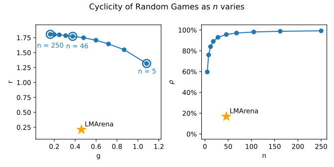
We compare the Hodge statistics of the real game against i.i.d. Uniform games of varying sizes. Results are plotted in Figure 1, averaged over \(1000\) runs. The left plot shows that as \(n\) grows, the gradient component of the random \(P\) decreases in strength while the strength of the rotational component increases. At comparable size \(n=46\), the two games have transitive strengths of the same order (\(g\approx.37\) for the random game against \(g=.46\) for the real one), but the rotational strength of the random game falls at \(1.77\), which is about 8.6x as strong as the real game’s \(r=.206\).
The right plot shows the trend of the Hodge ratio as a function of \(n\). As \(n\) grows, \(\rho\) quickly saturates to nearly \(100\%\). This is intuitive as the i.i.d. Uniform generator produces completely arbitrary order between every pair of responses, and the resulting preference matrix is thus almost entirely rotational. The real game, on the other hand, is remarkably transitive. Intuitively, it stems from the fact that there is a tangible difference in quality between many models selected, and some are just unequivocally better than others. There remains, though, an unexplained rotational component – \(16.8\%\) unweighted (or \(11.2\%\) weighted) – which reflects genuine intransitivity, noisiness from the dataset, or both.
4. Solve rate collapses with more cyclicity
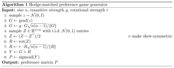
We design a synthetic game generator to remedy the mismatched transitive and rotational strengths of the i.i.d. Uniform generator. Algorithm 1 generates a preference game of any desired transitive strength \(g\) and rotational strength \(r\).
We investigate how the solve rates of OMD, NashMD and EGPO rely on the Hodge statistics by generating games of various \(g\) and \(r\). We consider a regularized game solved if the last-iterate duality gap falls below 1e-6 after a specified number of iterations (in this case, \(10000\)). We choose regularization strength \(\beta=.001\), a weak regularization, in order to avoid tampering with the cyclicity of the games. Learning rate \(\eta\) is tuned per-algorithm on a scale from \(.01\) to \(3\) to ensure that none of the algorithms are disadvantaged by a small learning rate.
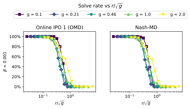
Figure 2 plots the solve rate of OMD and NashMD against an empirically chosen quantity \(r/\sqrt{g}\). It appears that neither \(r\) or \(g\) alone predicts how well the algorithms perform; the interaction between them does. With \(g\) fixed, a higher cyclicity makes it harder for OMD and NashMD to converge. On the other hand, with \(r\) fixed, a smaller \(g\) makes it harder for the algorithms to find the optimum, presumably because this translates to a weaker preference (that is, \(P_{ij}\) closer to \(0.5\)).
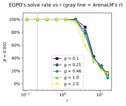
EGPO, however, appears to follow a different pattern unaffected by the transitive strength, as shown in Figure 3. The solve rate of EGPO remains consistent for all \(g\) up until \(r\approx 3\), where it begins to falter. It seems that EGPO is the more robust answer to high cyclicity compared to the other two algorithms: its solve rate stays at 100% beyond the \(r\) that makes OMD and NashMD collapse. At realistic \(r = .206\) and \(g=.458\) (that is, \(r/\sqrt{g} \approx .30\), marked by the gray line), however, all three algorithms still solve essentially every instance of the problem, so this robustness is not yet what separates them on real data.
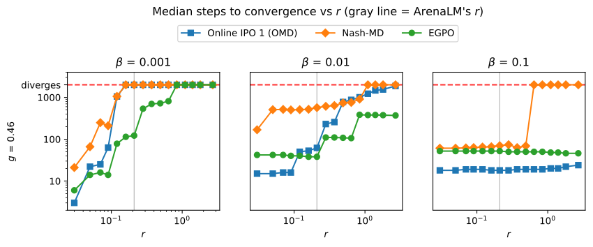
To further understand the effect of cyclicity, we fix \(g\) at realistic levels and plot the median steps to convergence (given that the run converges) against \(r\) for all three algorithms at three different regularization strengths. For each \(\beta\), a different iteration budget is given, with a larger \(\beta\) receiving fewer iterations. The results are plotted in Figure 4. In the rightmost plot with the heaviest regularization \(\beta=0.1\), OMD is the fastest to converge at every \(r\). For the other plots, OMD still wins at small \(r\) but starts to suffer as \(r\) grows larger, with EGPO overtaking it at around \(r\approx.1\) for \(\beta=.001\) and \(r\approx.2\) for \(\beta=.01\) – and past that point EGPO is the only one of the three that remains convergent. EGPO thus appears to be the insurance against high cyclicity, which is close to the regime Zhou et al. (2025) evaluate in: their tabular simulations draw \(P\) i.i.d. Uniform (a highly rotational game) and they report EGPO’s advantage to be largest at \(\beta=0.001\), their smallest regularization. NashMD is never the winner.
5. Do Hodge-matched games predict the real one?
There remains a question: do the results from the modified synthetic generator with matched Hodge statistics transfer to real preference data? We answer this by directly testing the three algorithms on the LMArena game at five different regularization levels from 1e-3 to 1e-1. The results are shown in Figure 5. Two observations jump out:
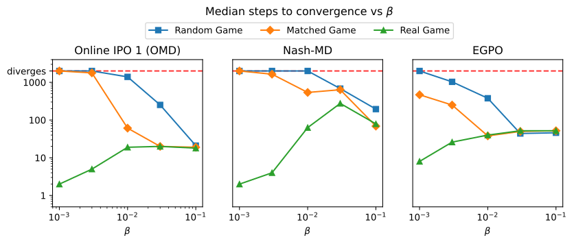
- Hodge-matched games reproduce real-game behavior only at large \(\beta\). In fact, at \(\beta \ge .01\), matched games track the median steps to convergence of the real game for EGPO almost exactly. At small \(\beta\), however, matched games fail in the same way i.i.d. Uniform games do.
- The trend in \(\beta\) is inverted. As regularization weakens, the matched generator predicts slower convergence, but on the real game the exact opposite happens. Indeed, the real game regularized at \(\beta = .001\) is solvable by OMD in two steps, while on matched games it diverges altogether. This suggests a structural mismatch between synthetic games and real games that the tabular benchmark doesn’t capture. One hypothesis is that real preference data is fundamentally easy to solve in a way not described by Hodge statistics, and this easiness is what powers the empirical success of transitivity-based models like PPO and DPO in practice.
6. Conclusion and Limitations
We investigated the effect of transitivity and cyclicity of the regularized preference game on three NLHF algorithms and conclude that at the cyclicity level that real data exhibits, OMD dominates on steps to convergence; while EGPO pays off only under small \(\beta\) and large \(r\). We propose a modified synthetic game generator and find that while it improves over the i.i.d. Uniform generator at large \(\beta\), matching Hodge statistics is insufficient at small \(\beta\).
We identify the following limitations to our approach:
- We have only investigated the exact tabular setting, not the sampled or the neural network setting more realistic to RLHF.
- We did not isolate the effect of noise in generating the preference data. The gap between the unweighted and Fisher-weighted Hodge ratios suggests that a meaningful part of the measured cyclicity is sampling artifact rather than genuine intransitivity, and a real game’s rotational strength may therefore sit below even our weighted estimate.
- In RLHF, the preference game’s actions are responses to a fixed prompt, while our LMArena matrix are different models over a prompt distribution. Aggregating over different models might not make sense in the same way that mixing the parameters \(\theta\) of a tabular softmax policy does.
References
David Balduzzi, Karl Tuyls, Julien Pérolat, and Thore Graepel. 2018. “Re-evaluating Evaluation.” Advances in Neural Information Processing Systems 31. arXiv:1806.02643.
Ralph Allan Bradley and Milton E. Terry. 1952. “Rank Analysis of Incomplete Block Designs: I. The Method of Paired Comparisons.” Biometrika 39 (3/4): 324–345. doi:10.1093/biomet/39.3-4.324.
Daniele Calandriello, Daniel Guo, Rémi Munos, Mark Rowland, Yunhao Tang, Bernardo Ávila Pires, Pierre Harvey Richemond, Charline Le Lan, Michal Valko, Tianqi Liu, Rishabh Joshi, Zeyu Zheng, and Bilal Piot. 2024. “Human Alignment of Large Language Models through Online Preference Optimisation.” arXiv:2403.08635.
Wojciech M. Czarnecki, Gauthier Gidel, Brendan Tracey, Karl Tuyls, Shayegan Omidshafiei, David Balduzzi, and Max Jaderberg. 2020. “Real World Games Look Like Spinning Tops.” Advances in Neural Information Processing Systems 33. Proceedings page.
Xiaoye Jiang, Lek-Heng Lim, Yuan Yao, and Yinyu Ye. 2011. “Statistical Ranking and Combinatorial Hodge Theory.” Mathematical Programming 127: 203–244. doi:10.1007/s10107-010-0419-x.
Alexander Y. Klimenko. 2015. “Intransitivity in Theory and in the Real World.” Entropy 17 (6): 4364–4412. doi:10.3390/e17064364.
LMArena. 2024. “arena-human-preference-140k.” Hugging Face dataset. Dataset card.
Kenneth O. May. 1954. “Intransitivity, Utility, and the Aggregation of Preference Patterns.” Econometrica 22 (1): 1–13. doi:10.2307/1909827.
Rémi Munos, Michal Valko, Daniele Calandriello, Mohammad Gheshlaghi Azar, Mark Rowland, Zhaohan Daniel Guo, Yunhao Tang, Matthieu Geist, Thomas Mesnard, Andrea Michi, Marco Selvi, Sertan Girgin, Nikola Momchev, Olivier Bachem, Daniel J. Mankowitz, Doina Precup, and Bilal Piot. 2023. “Nash Learning from Human Feedback.” arXiv:2312.00886.
Rafael Rafailov, Archit Sharma, Eric Mitchell, Stefano Ermon, Christopher D. Manning, and Chelsea Finn. 2023. “Direct Preference Optimization: Your Language Model Is Secretly a Reward Model.” Advances in Neural Information Processing Systems 36. Proceedings page.
John Schulman, Filip Wolski, Prafulla Dhariwal, Alec Radford, and Oleg Klimov. 2017. “Proximal Policy Optimization Algorithms.” arXiv:1707.06347.
Csaba Szepesvári. 2026. “Applications of RL in Production.” Presentation slides. Google Slides.
Runlong Zhou, Maryam Fazel, and Simon S. Du. 2025. “Extragradient Preference Optimization (EGPO): Beyond Last-Iterate Convergence for Nash Learning from Human Feedback.” arXiv:2503.08942.
Appendix: computing the Hodge decomposition
The score minimization problem is convex and has a closed-form solution. The solution is \(s = L^{+}b\), where
\[L := \operatorname{diag}(W\mathbf{1}) - W, \quad b_i := \sum_j w_{ij}Y_{ij},\]and \(L^{+}\) denotes the Moore-Penrose pseudoinverse. \(L\) is known as the weighted graph Laplacian. The gradient and rotational parts are then \(G = \operatorname{grad}(s)\) and \(R = Y - G\).
It should be noted that at no point in the definition of the Hodge decomposition are the diagonal entries of \(W\) used (they’re undefined). Hence we enforce \(W_{ii}=0\) in the following code for simplicity. Uniform weighting is expressed by W=None. Computations are batched over the first axis.
def grad(s):
    """G = s1ᵀ - 1sᵀ, i.e. G[i,j] = s[i] - s[j]."""
    s = np.asarray(s)
    return s[..., :, None] - s[..., None, :]


def inner(A, B, W=None):
    """⟨A, B⟩_W = Σ W[i,j] A[i,j] B[i,j]."""
    if W is None:
        return np.sum(A * B, axis=(-2, -1))
    return np.sum(A * B * W, axis=(-2, -1))


def decompose(Y, W=None):
    """
    Decompose skew-symmetric Y = G + R, where
    ⋅ s is the score vector,
    ⋅ G = grad(s) = s1ᵀ - 1sᵀ is the gradient part,
    ⋅ R is the rotation part,
    ⋅ G, R are both skew-symmetric,
    ⋅ ⟨G, R⟩_W = 0,
    ⋅ ‖G‖_W² + ‖R‖_W² = ‖Y‖_W².
    """
    Y = np.asarray(Y)

    assert Y.shape[-1] == Y.shape[-2], "Y must be square"
    assert np.allclose(
        Y + np.swapaxes(Y, -1, -2),
        0,
        atol=1e-6,
    ), "Y must be skew-symmetric"

    n = Y.shape[-1]

    if W is not None:
        W = np.asarray(W)

        assert W.ndim == 2, "W must be a matrix"
        assert W.shape[0] == W.shape[1], "W must be square"
        assert W.shape == Y.shape[-2:], "Y and W must have the same matrix shape"
        assert np.allclose(W, W.T), "W must be symmetric"
        assert np.all(W >= 0), "W must be nonnegative"
        assert np.allclose(np.diag(W), 0), "The diagonal of W must be 0"
    else:
        W = np.ones((n, n)) - np.eye(n)

    # Weighted graph Laplacian
    L = -W.copy()
    np.fill_diagonal(L, W.sum(axis=-1))

    b = np.sum(W * Y, axis=-1)

    s = b @ np.linalg.pinv(L)

    G = grad(s)
    R = Y - G
    # Optional: return Hodge ratio too
    # rho = inner(R, R, W) / inner(Y, Y, W)

    return G, R  #, rho